Getting and plotting real-time traffic data

visualization

hereR

traffic

Using {hereR} to get live speed

Published

September 23, 2023

This post introduces you to the hereR package that enables you to get real-time speed (and other) data via the HERE Traffic API. I will be requesting data for the cities of Windsor and Toronto in Ontario, Canada.

Requesting data via the API requires an API key that you can create as described in the instructions. Once you get and set the api_key, you are ready to request the data. Note that there is a rate limit to how much data you can request everyday.

Let’s start by loading the package:

library(hereR)

Getting the spatial polygons of cities

The hereR package requires spatial polygons of the areas for which the traffic data is requested. Therefore, the first step is to get the bounding boxes of Windsor and Toronto via the osmdata package:

library(osmdata)

city1 <- "Windsor, Ontario"
city2 <- "Toronto, Ontario"

bbox1 <- getbb(city1)
bbox2 <- getbb(city2)

# Windsor bounding box
print(bbox1)

        min       max
x -83.19734 -82.87734
y  42.15674  42.47674

Next, we get the spatial data for Ontario via the geodata package:

library(geodata)
library(sf)

cdn <- geodata::gadm(country = "can", level = 1, path = tempdir())
ont <- cdn[9,]

ont <- st_as_sf(ont)
ont

Simple feature collection with 1 feature and 11 fields
Geometry type: MULTIPOLYGON
Dimension:     XY
Bounding box:  xmin: -95.15598 ymin: 41.67693 xmax: -74.34605 ymax: 56.86972
Geodetic CRS:  WGS 84
    GID_1 GID_0 COUNTRY  NAME_1    VARNAME_1 NL_NAME_1   TYPE_1 ENGTYPE_1 CC_1
1 CAN.9_1   CAN  Canada Ontario Upper Canada      <NA> Province  Province   35
  HASC_1 ISO_1                       geometry
1  CA.ON CA-ON MULTIPOLYGON (((-78.91332 4...

As you can see, ont is a simple feature (sf) object with geometry type of multipolygon. Bounding boxes can now be used to extract the data for the two cities only:

windsor <- st_crop(ont, 
                  xmin=bbox1[1, 1],
                  xmax=bbox1[1, 2],
                  ymin=bbox1[2, 1],
                  ymax=bbox1[2, 2])

toronto <- st_crop(ont, 
                   xmin=bbox2[1, 1],
                   xmax=bbox2[1, 2],
                   ymin=bbox2[2, 1],
                   ymax=bbox2[2, 2])

toronto

Simple feature collection with 1 feature and 11 fields
Geometry type: POLYGON
Dimension:     XY
Bounding box:  xmin: -79.49282 ymin: 43.61038 xmax: -79.27851 ymax: 43.73602
Geodetic CRS:  WGS 84
    GID_1 GID_0 COUNTRY  NAME_1    VARNAME_1 NL_NAME_1   TYPE_1 ENGTYPE_1 CC_1
1 CAN.9_1   CAN  Canada Ontario Upper Canada      <NA> Province  Province   35
  HASC_1 ISO_1                       geometry
1  CA.ON CA-ON POLYGON ((-79.49282 43.6103...

Requesting the traffic data

Now we are ready to request the traffic data via the flow function from the hereR package:

flows_windsor <- flow(aoi = windsor)
flows_toronto <- flow(aoi = toronto)

head(flows_windsor)

Simple feature collection with 6 features and 7 fields
Geometry type: MULTILINESTRING
Dimension:     XY
Bounding box:  xmin: -83.06751 ymin: 42.23461 xmax: -82.95438 ymax: 42.31681
Geodetic CRS:  WGS 84
  id     speed speed_uncapped free_flow jam_factor confidence traversability
1  1 12.777778      12.777778 12.500000          0       0.70           open
2  1 15.277779      18.333334 14.444445          0       0.77           open
3  1 13.888889      15.000000 13.333334          0       0.76           open
4  1 11.111112      11.111112  5.555556          0       0.70           open
5  1  8.611112       8.611112  8.611112          0       0.70           open
6  1 29.166668      29.166668 22.222223          0       0.70           open
                        geometry
1 MULTILINESTRING ((-83.02933...
2 MULTILINESTRING ((-83.00378...
3 MULTILINESTRING ((-82.99749...
4 MULTILINESTRING ((-82.95438...
5 MULTILINESTRING ((-83.04222...
6 MULTILINESTRING ((-83.06751...

Cool. As you can see, the returned data is also of type sf but with many variables. Following table contains the descriptions of these variables (source).

Variable	Description	Units
speed	The average speed, capped by the speed limit, that current traffic is travelling.	meters per second
speedUncapped	The average speed, not capped by the speed limit, that current traffic is travelling.	meters per second
freeFlow	The free flow speed speed is a reference speed provided to indicate the speed on the segment at which vehicles should be considered to be able to travel without impediment.	meters per second
jamFactor	The number between 0.0 and 10.0 indicating the expected quality of travel. When there is a road closure, the `jamFactor` will be 10.0. As the value approaches 10.0 the quality of travel is getting worse.
confidence	The number between 0.0 and 1.0 indicating the proportion of real time data included in the speed calculation. 0.7 < `confidence` <= 1.0 indicates real time speeds 0.5 < `confidence` <= 0.7 indicates historical speeds 0.0 < `confidence` <= 0.5 indicates speed limit This field can be used to identify whether the data for a location is derived from real time probe sources or historical information only. All confidence data 0.71 and above is based on real-time information, where a confidence value of 0.75 or greater indicates high confidence real-time information. A confidence value equal to 0.70 means that the data is derived from historical data only.
traversability	“open” / “closed” / “reversibleNotRoutable” Indicates whether this roadway can be driven.

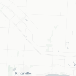
Plotting speed and jam factor

Following plots show the speed and jam factor side-by-side for Windsor, Ontario roads at 2023-09-23 23:29:40. These are interactive maps: You can zoom in/out, hover over or click on the roads to get more information.

Windsor

Show the code

library(mapview)
library(leaflet)
library(leafpop)
library(leafem)
library(raster)
library(leafsync)

m1 <- mapview(flows_windsor,
  popup = popupTable(flows_windsor,
    zcol = c(
      "free_flow",
      "speed",
      "jam_factor",
      "confidence"
    )
  ),
  zcol = "speed",
  layer.name = "speed"
)


m2 <- mapview(flows_windsor,
  popup = popupTable(flows_windsor,
    zcol = c(
      "free_flow",
      "speed",
      "jam_factor",
      "confidence"
    )
  ),
  zcol = "jam_factor",
  layer.name = "jam_factor"
)

sync(m1, m2)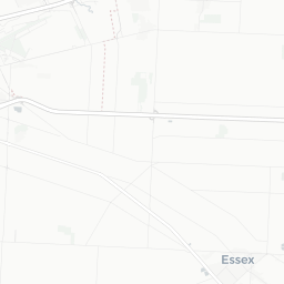

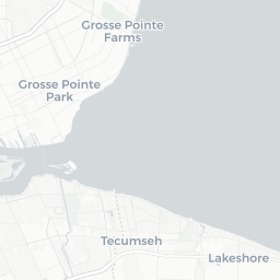
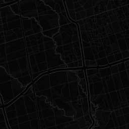
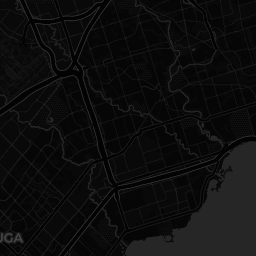
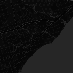
Toronto

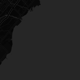
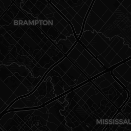
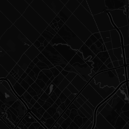
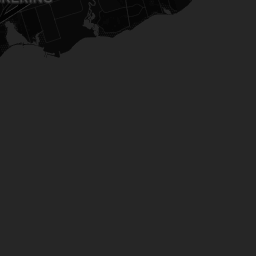
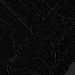
Following uses a different base map with Toronto speeds:

Show the code

mapview(flows_toronto,
  popup = popupTable(flows_toronto,
    zcol = c(
      "free_flow",
      "speed",
      "jam_factor",
      "confidence"
    )
  ),
  zcol = "speed",
  layer.name = "speed",
  map.types = c("CartoDB.DarkMatter"),
  homebutton = FALSE
) %>%
  leafem::addHomeButton(ext = extent(toronto), group = "Toronto")

This workflow can be scaled to larger number of cities and days with the power of Github Actions to get traffic data every day, month, etc.