suppressPackageStartupMessages( library(tidyverse) )
suppressPackageStartupMessages( library(here) )
suppressPackageStartupMessages( library(readr) )Draw cars with ggplot2
Credit:
Thanks to BrodieG for answering my stackoverflow question about drawing diagrams in R.
I wanted to draw cars
I wanted to plot a car following another car using ggplot2. There are geom_rect and geom_tile that could do that, but I wanted to give the rectangles a ‘car’ look. So, I posted a question on stackoverflow (linked above). The answer showed how to do that by creating a geom_car
Creating geom_car
Creating a new geom in ggplot2 is much more complicated then using the ggplot2 interface. The official gpplot2 book, ggplot2: Elegant Graphics for Data Analysis, says the following:
When making the jump from user to developer, it is common to encounter frustrations because the nature of the ggplot2 interface is very different to the structure of the underlying machinery that makes it work
And I completely agree. The chapter that the above quote is from explains that ggplot2 uses the ggproto class system to create new objects such as geoms.
The following shows the use of ggproto that creates the geom_car. Again, the code is not mine but provided by Brodie G (thanks!).
First, load libraries.
Load Libraries
Load data
I am using a dataset of 2 cars. The Following car is approaching a Lead car from a large distance. The Lead car is stopped. The dataset contains the x and y coordinates of the centroid of cars and their sizes.
df <- read_csv("driver_data.csv")Rows: 49 Columns: 12
── Column specification ────────────────────────────────────────────────────────
Delimiter: ","
dbl (12): Time_s, ED_x_m, ED_y_m, LV_x_m, LV_y_m, LV_length_m, LV_width_m, v...
ℹ Use `spec()` to retrieve the full column specification for this data.
ℹ Specify the column types or set `show_col_types = FALSE` to quiet this message.head(df)# A tibble: 6 × 12
Time_s ED_x_m ED_y_m LV_x_m LV_y_m LV_length_m LV_width_m visual_angle_W
<dbl> <dbl> <dbl> <dbl> <dbl> <dbl> <dbl> <dbl>
1 1 4341. -8921. 3991. -7732. 5.39 2.29 0.00185
2 2 4335. -8899. 3991. -7732. 5.39 2.29 0.00189
3 3 4329. -8877. 3991. -7732. 5.39 2.29 0.00193
4 4 4322. -8854. 3991. -7732. 5.39 2.29 0.00197
5 5 4315. -8831. 3991. -7732. 5.39 2.29 0.00201
6 6 4308. -8808. 3991. -7732. 5.39 2.29 0.00205
# ℹ 4 more variables: visual_angle_H <dbl>, tau <dbl>, ED_length_m <dbl>,
# ED_width_m <dbl>Coordinates plot
Following plot shows that in the original data format, the Following car moves up and left towards the lead car.
ggplot(data = df,
       aes(x = ED_x_m, y = ED_y_m)) +
  geom_line(aes(color = "Following car"))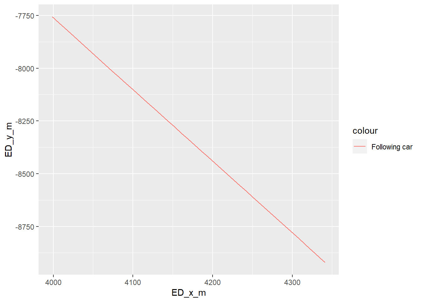
Step 1: Create a car image with no fill color
The stackoverflow answer comes with a car image, but I wanted to experiment with my own image. So, I created one with no fill color. This was important to enable the fill method in geom_car. Then it was read by the png::readPNG method:
car.raster <- png::readPNG("car4.png")

str(car.raster)
num [1:238, 1:505, 1:4] 0 0.184 0.184 0.184 0.184 ...Step 2: Create a graphical object (grob) from the image
# Generate a car 'grob' using a baseline PNG

# The `grid` grob actually responsible for rendering our car,
# combines our transparent car elements with a background rectangle
# for color/fill.

carGrob <- function(x, y, length, width, gp) {
  grid::grobTree(
    grid::rectGrob(
      x, y, hjust=.5, height=width, width=length,
      gp = gp
    ),
    grid::rasterGrob(
      car.raster, x=x, y=y, hjust=.5, height=width, width=length
    ) ) }
Step 3: Map the data to the grob using ggproto
# The `ggproto` object that maps our data to the `grid` grobs

GeomCar <- ggplot2::ggproto("GeomCar", ggplot2::Geom,
                            # Generate grobs from the data, we have to reconvert length/width so
                            # that the transformations persist

                            draw_panel=function(self, data, panel_params, coords) {
                              with(
                                coords$transform(data, panel_params),
                                carGrob(
                                  x, y, length=xmax-xmin, width=ymax-ymin,
                                  gp=grid::gpar(
                                    col = colour, fill = alpha(fill, alpha),
                                    lwd = size * .pt, lty = linetype, lineend = "butt"
                                  ) ) ) },
                            # Convert data to coordinates that will get transformed (length/width don't
                            # normally).

                            setup_data=function(self, data, params) {
                              transform(data,
                                        xmin = x - length / 2, xmax = x + length / 2,
                                        ymin = y - width / 2, ymax = y + width / 2
                              ) },
                            # Required and default aesthetics

                            required_aes=c("x", "y", "length", "width"),
                            default_aes = aes(
                              colour = NA, fill = "grey35", size = 0.5, linetype = 1, alpha = NA
                            ),
                            # Use the car grob in the legend

                            draw_key = function(data, params, size) {
                              with(
                                data,
                                carGrob(
                                  0.5, 0.5, length=.75, width=.5,
                                  gp = grid::gpar(
                                    col = colour, fill = alpha(fill, alpha),
                                    lwd = size * .pt, lty = linetype, lineend = "butt"
                                  ) ) ) }
)
Step 4: Create the external interface i.e. the geom_car layer
# External interface

geom_car <- function(
  mapping=NULL, data=NULL, ..., inherit.aes=TRUE, show.legend=NA
) {
  layer(
    data=data, mapping=mapping, geom=GeomCar, position="identity",
    stat="identity", show.legend = show.legend, inherit.aes = inherit.aes,
    params=list(...)
  )
}
Plotting the cars
I can now use geom_car to plot the cars. Since the coordinates change every second (see the Time_s column above), I need to filter for one time only. So, I choose Time_s == 49.
Attempt 1 to plot cars
ggplot(df %>% filter(Time_s == 49) ) +
  geom_car(aes(x=ED_x_m, y=ED_y_m,
               length=ED_length_m, width=ED_width_m,
               fill="ed")) +
  geom_text(aes(x=ED_x_m, y=ED_y_m+5),
            label = "Following Car") +

  geom_car(aes(x=LV_x_m, y=LV_y_m,
               length=LV_length_m, width=LV_width_m,
               fill="lv")) +
  geom_text(aes(x=LV_x_m, y=LV_y_m+5),
            label = "Lead Car\n(stationary)") +

  coord_equal(ratio = 0.7) +
  theme(legend.position = "none")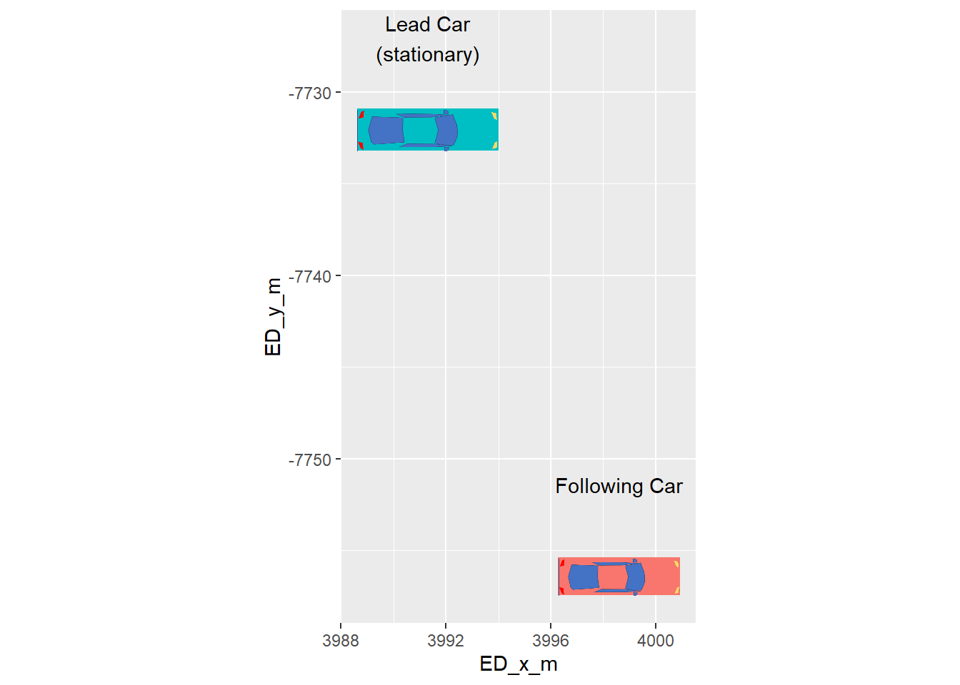
This does not look right. The Following car seems to be ahead of the lead car. Also, due to the elongated scale, the Following car appears to be in a different lane. The main reason is the unusual coordinates. The x coordinates decrease as the Following car gets closer to the lead car.
I can fix this by scaling: subtracting the x coordinates from the largest x coordinate in the data.
Attemp 2: Adjust the coordinates and plot again
Adjust coordinates:
first_ed_x_coord <- df %>% pull(ED_x_m) %>% range() %>% tail(1)

df <- df %>%
  mutate(
    ED_x_m_a = abs(ED_x_m - first_ed_x_coord),
    LV_x_m_a = abs(LV_x_m - first_ed_x_coord)
         )
Plot:
ggplot(df %>% filter(Time_s == 49) ) +
  geom_car(aes(x=ED_x_m_a, y=ED_y_m,
               length=ED_length_m, width=ED_width_m,
               fill="ed")) +
  geom_text(aes(x=ED_x_m_a, y=ED_y_m+5),
            label = "Following Car") +

  geom_car(aes(x=LV_x_m_a, y=LV_y_m,
               length=LV_length_m, width=LV_width_m,
               fill="lv")) +
  geom_text(aes(x=LV_x_m_a, y=LV_y_m+5),
            label = "Lead Car\n(stationary)") +

  coord_equal(ratio = 0.7) +
  theme(legend.position = "none")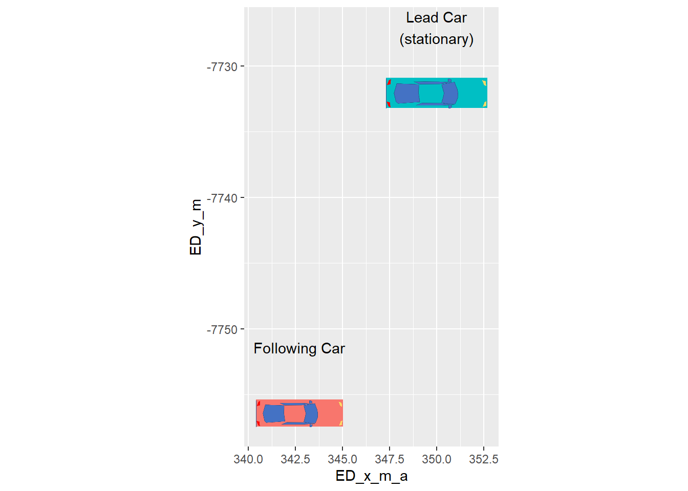
This is better. Now, to fix the problem of the elongated y coordinate, I can fix them to a single value, because I’m mainly interested in the movement along the x-axis. But note that this might not be a good idea if there is a large change in y coordinate (e.g. in a lane change).
Attempt 3 - Fixing y coordinate
car_plot <- ggplot(df %>% filter(Time_s == 49) ) +
  geom_car(aes(x=ED_x_m_a, y=300,
               length=ED_length_m, width=ED_width_m,
               fill="ed")) +
  geom_text(aes(x=ED_x_m_a, y=300+5),
            label = "Following Car") +

  geom_car(aes(x=LV_x_m_a, y=300,
               length=LV_length_m, width=LV_width_m,
               fill="lv")) +
  geom_text(aes(x=LV_x_m_a, y=300+5),
            label = "Lead Car\n(stationary)") +
  theme_void() +
  coord_equal(ratio = 1) +
  theme(legend.position = "none",
        axis.text = element_blank(),
        axis.title = element_blank(),
        axis.ticks = element_blank())

car_plot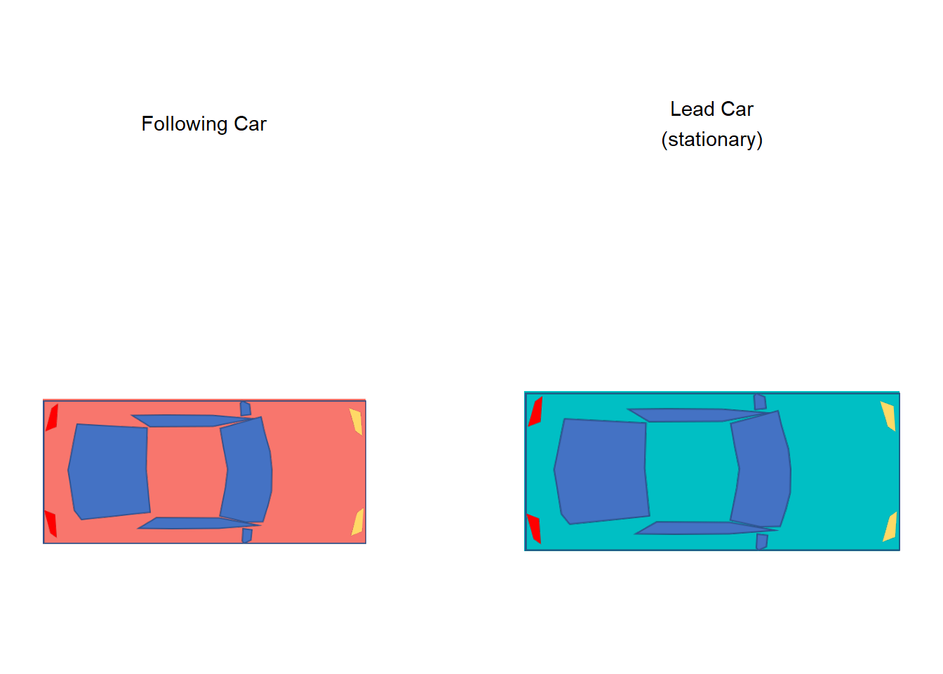
This looks much better. :D
Car Rear View
I also created a geom_car_rear by using a different image (car rear created in powerpoint). Following plots the car rear at time = 49 s.
ggplot(df %>% filter(Time_s == 49)) +
  geom_car_rear(aes(x=0, y=0, length=visual_angle_W,
               width=visual_angle_H), fill="black") +
  theme_void()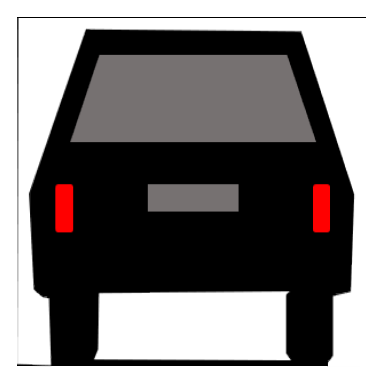
Bonus: Animation
Since I have data across time, I can also animate my cars using the fantastic gganimate package. Here goes:
library(gganimate)

ggplot(df ) +
  geom_car(aes(x=ED_x_m_a, y=300,
               length=ED_length_m, width=ED_width_m,
               fill="ed")) +
  geom_text(aes(x=ED_x_m_a, y=300+5),
            label = "Following Car") +

  geom_car(aes(x=LV_x_m_a, y=300,
               length=LV_length_m, width=LV_width_m,
               fill="lv")) +
  geom_text(aes(x=LV_x_m_a, y=300+5),
            label = "Lead Car\n(stationary)") +
  theme_void() +
  coord_equal(ratio = 1) +
  theme(legend.position = "none",
        axis.text = element_blank(),
        axis.title = element_blank(),
        axis.ticks = element_blank())  +
  transition_time(Time_s) +
  view_follow()
This animation has one limitation. The lead car also appears to be moving. Maybe putting a vertcial line or using gganimate::view_step() might solve this problem. I’d perhaps explore that in a different post.